Introduction | Tank – How to | Tank – Examples | Atmosphere – The Polar Front | Atmosphere – Synoptic Fronts | Theory | For Teachers | Wiki
Previously performed cylinder collapse experiment
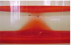
Have a look at the sequence of pictures below. They show the top view of the cylinder collapse experiment. Note how we use a mirror (at the top) inclined at 45 degrees to reveal the vertical structure of the slumping cone of salty water. A video capturing this sequence can be downloaded here. Note that the video is recorded by a camera rotating with the tank.
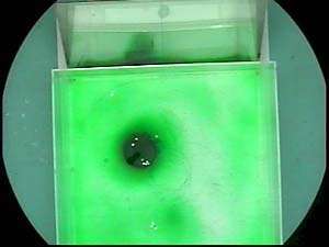
We observe that paper dots floating on the surface far away from the cone, move more slowly than dots closer to the cone. This is consistent with the thermal wind relation which tells us that large horizontal density gradients, which exist close to the cone, are associated with a large vertical shear of the geostrophic flow (see here for background theory). Because the flow near the bottom of the tank feels bottom drag, currents at the surface revealed by floating paper dots move more rapidly.
The state of affairs is shown schematically below: paper dots placed on the surface directly above the edge of the cone that is sloping the most steeply, swirl the fastest. Paper dots placed far away from the cone where the slope of the front is close to zero move only very slowly relative to the rotating tank.

Quantitative estimates for the experiment
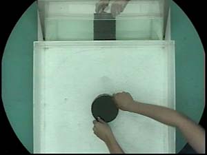
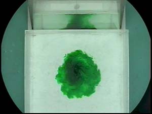
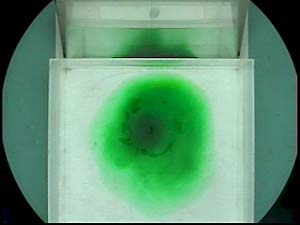
The paper dots can be tracked using ‘particle tracking’ software as in the example below, enabling their speed to be determined, and the density of the salty water measured from a sample extracted using a syringe.
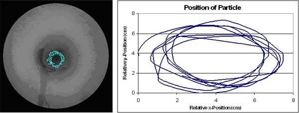
Once estimates of particle velocities and density of the salty water are obtained (approximately 8 cm s-1 and 1.06 g cm-3, respectively, in the above example), we can use Margules relation (see theory), reproduced below, to predict the slope of the frontal surface directly below the swirling particle:
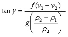
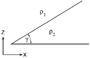
Here region 1 is the lighter fluid and region 2 is the denser fluid. The Coriolis parameter, f, for the above experiment is 2Ω, and γ is the angle of the frontal surface, as sketched below.
Note that we assume v2, the component of the current parallel to the front in the denser fluid, is much smaller than that of v1. Using the Margules relation and the measured values given above (be careful to express the rotation rate in terms of radians per second!), the predicted angle of the front is 28°. Comparing this to the observed slope of the front below the left-most particle in the photo below, we obtain 33°, perhaps a fortuitously close agreement!