Introduction | Tank – How to | Tank – Examples | Atmosphere – The Polar Front | Atmosphere – Synoptic Fronts | Theory | For Teachers | Wiki
 In the atmosphere, the transition from warm, equatorial air to cold polar air is not gradual, but occurs rather abruptly in mid-latitudes where tropical and polar air masses meet at the polar front. Everyday weather is often associated with undulations of this frontal surface. Here we will study the observed structure of the polar front.
On the right you can see the long-term Northern Hemisphere mean air temperature at 500mb for January, contoured every 5°C. Note that the temperature gradient is strongest in mid-latitudes, and marks the location of the polar front. You can make your own plots here.
A cross-section of the temperature field shown below running from the equator (left) to the pole (right) at 150°E shows the location of the polar front for January conditions, stretching from the equator to the north pole. Note the sudden drop in temperature between 30-40°N.
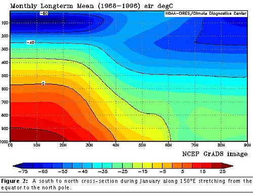
For a 3D view of the polar front see here.
Thermal Wind Equation
According to the thermal wind equation, horizontal temperature gradients are associated with vertical wind shear. Therefore, we expect to see vertical wind shear in the region of strongest temperature gradient, as you can see below in the figure illustrating the climatological zonal component of the wind normal to the 150°E profile as the figure above.
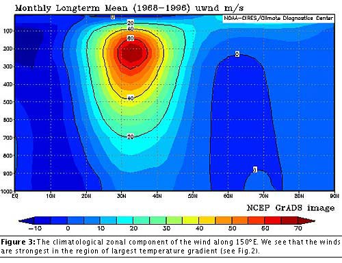
The thermal wind equation in pressure coordinates can be written
where the meridional temperature gradient is carried out at constant pressure. Here R = 287J kg-1K-1 is the gas constant and f = 2Ωsinφ is the Coriolis parameter where Ω=7.29×10⁻⁵ s-1 and φ is latitude. Noting that one degree of latitude is about 110 km, we can use the data plotted in the above two firgures to quantitatively check the above balance.
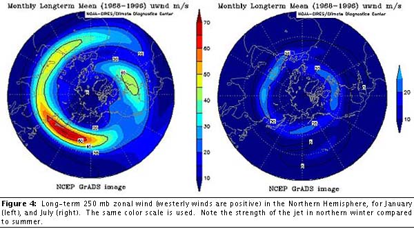
The climatological jet in both hemispheres is primarily westerly, i.e. from west to east. The temperature gradient that is associated with the jet, however, is greater during the winter than in summer because of the seasonal cycle in solar heating. Accordingly, the jet is also stronger in the winter as shown in the diagrams below, where long-term 250 mb zonal wind (westerly winds are positive) in the Northern Hemisphere, for January are shown on the left, and for July on the right. The same color scale is used. Note the strength of the jet in northern winter compared to summer.
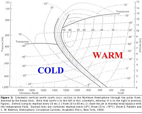
Combining our observations of air temperature and zonal wind, the polar front can be schematically represented in a vertical north-south cross section of the Northern Hemisphere through the polar front, denoted by the heavy lines. Note that north is to the left in this diagram, whereas it is to the right in figures above. Dotted isotachs marked every 10 m/s (from 10 to 80 m/s) show the jet in thermal wind balance with the temperature field. Dashed lines are isotherms marked every 10C (from 10 to -70°C). (from E. Palmen and C. W. Newton, Atmospheric Circulation Systems, Academic Press, New York, 1969)
Slope of Frontal Surface following Margules
From the diagram above, we can see that the polar front has a distinct slope, just as seen in our laboratory experiment. We can use the Margules relation to predict the slope of the front from observations of winds and temperatures:
where we have assumed that T1~ T2 ~T (see theory for a discussion of the Margules relation). Taking T to be about 260K, latitude to be 45°N, and using the above figure, we can estimate the slope of the polar front using the above formula. This should be compared to the observed slope.
Southern Hemisphere
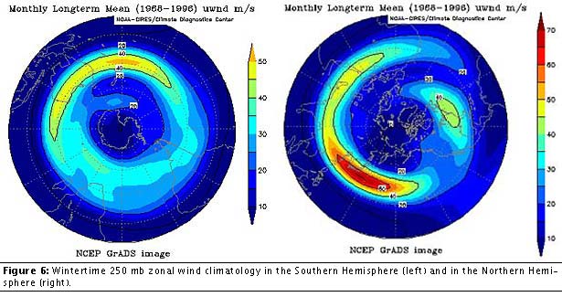
There is less land in the Southern Hemisphere than in the Northern Hemisphere, and so fewer processes are present to create zonal inhomogeneities. Consequently, the jet-stream in the Southern Hemisphere is more symmetric than in the north as can be seen in the diagrams below which show wintertime 250 mb zonal wind climatology in the Southern Hemisphere (left) and in the Northern Hemisphere (right).
It is instructive to create your own cross-sections through the polar front at a longitude other than 150°E. Check for thermal wind balance and use Margules relation to interpret the slope of the frontal surfaces.