Introduction | Tank – Hadley | Tank – Eddies | Atmosphere – Hadley | Atmosphere – Eddies | Theory | For Teachers | Wiki
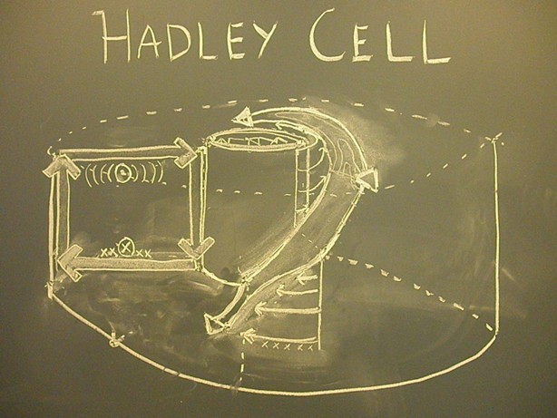
Hadley circulation (slow rotation): An ice bucket placed in the center of a rotating tank of water readily induces a radial temperature gradient analogous to that created on earth by differential heating which warms the equator and cools the pole. If the turntable is rotated very slowly an axisymmetric Hadley circulation is set up.
How to carry out the Slow Rotation experiment
It is straightforward to obtain a steady, axially-symmetric circulation driven by radial temperature gradients in our laboratory tank, a useful analogue of the Hadley Circulation. Ice placed in a metal bucket at the center of a rotating tank will induce a radial temperature gradient, and in the case of slow rotation, an azimuthal current and an associated overturning circulation in the radial plane.
We take our clear 16”x16” square container with its circular insert and place it dead center on a white board on the turntable. We fill it with water to a depth of 10 cm or so. At the center of the tank we place an open can of 10cm diameter weighted down to prevent it from floating away. The turntable is then set in to rotation at a speed of 1-2rpm (even less if possible) and left for 10 minutes or so until it has come in to solid body rotation.
The can is then filled with ice and topped up with water to flush out all air pockets and ensure good thermal conduction between the ice and the sides of the can. In this manner, water adjacent to the can is cooled, inducing a substantial radial temperature gradient.
The tank is then left for a few minutes for the circulation to develop before the experiment proper begins.
The flow can be visualized by:
- dropping in a few permanganate crystals roughly halfway from the center, which streak the vertical column and settle on the bottom. These give an indication of the flow in the bottom boundary layer
- black paper dots floating on the surface reveal the surface flow.
- colored dye can be injected at various points. But be sparing with the dye.
For quantitative calculations the paper dots can be tracked with a particle tracker and thermistors attached to data loggers can be placed near the can (e.g. three arranged vertically up the side of the can and two radially outward along the bottom) to determine vertical and radial temperature gradients.
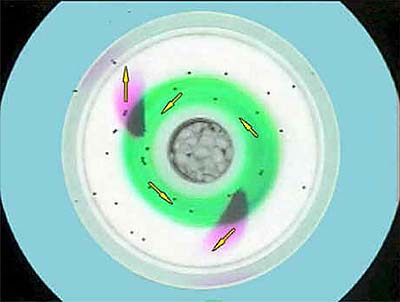
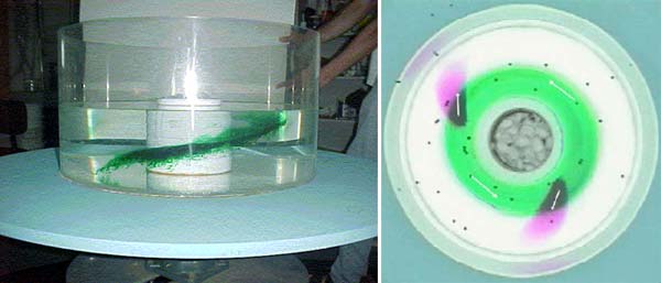
The photograph below is a top view of the tank in the Hadley regime (i) pink permanganate streaks reveal the flow at the bottom, (ii) green dye maps out the interior flow and (iii) black paper dots map the surface flow.
Previously Performed Experiments
In this experiment, cold water – made cold by the proximity of the ice bucket – sinks and flows radially outwards along the bottom. In compensation, relatively warm water rises and moves inward in the upper layers. Because of the presence of ambient rotation (due to the gentle cyclonic rotation of the turntable), the rings of fluid moving in to the center, spin more cyclonically as their radius decreases. Beneath, as rings of fluid expand on moving outwards, they acquire an anti-cyclonic spin. The figure below is a schematic diagram of the sense of the radial and azimuthal currents set up in the Hadley experiment.
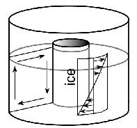
To help visualize the flow, we can drop in a few permanganate crystals which streak the vertical column and settle on the bottom. The streaks do not remain vertical; rather they tilt over in an azimuthal direction, carried along by the currents which increase in strength with height in a cyclonic sense (anticlockwise looking down) relative to the tank. This vertical current shear is a consequence of thermal wind, i.e. the radial temperature gradient.
The permanganate crystals on the bottom indicate the sense of flow right at the bottom. We see flow moving radially outwards and being deflected in an anticyclonic sense (clockwise looking down). Note the pink streamers moving outward and clockwise in the figure below, right. This flow is directly analogous to the trade winds of the atmosphere.
Green dye injected in to the flow, reveals the sense of the interior circulation (see below left). Black paper dots floating on the surface move in the same sense as, but more swiftly than, the rotating table. We have generated westerly (to the east) winds, a laboratory analogue of the subtropical jet.
View a movie of this experiment here.
Below are photographs revealing typical circulation patterns in the Hadley regime. Dye streaks (left) are tilted over by the cyclonic azimuthal current forming a beautiful cork-screw pattern. Flow in the bottom boundary layer, revealed by pink potassium permanganate streaks (right), is outward and anti-cyclonic.
Thermal Wind balance
As described above, we observe the development of an axisymmetric circulation in thermal wind balance with the radial temperature gradient in the Hadley experiment. For an incompressible fluid such as water, the thermal wind relation takes the form
where u is the azimuthal current, z is a vertical coordinate increasing upwards, α is the coefficient of expansion of water, g is gravity, Ω is the rate of rotation of the tank, T is temperature and r is the radius.
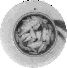
To quantitatively check the above balance, particle tracking software can be used to calculate the speed of a paper dot at the surface near the edge of the can (see below) and observations of temperature from thermisters. Note that we have to make some assumption about the speed of the current at the bottom of the tank (i.e.that it is somewhat smaller than at the surface). This can be checked by inspection of the movement of the pink streaks emanating from the permanganate crystals on the bottom. As illustrated below tracking paper dots floating on the surface can be used to determine flow speeds.
In a typical experiment, the rotation rate is 1 rpm (Ω = 0.1 rad s-1) and the water depth is 10cm. Typical surface current speeds close to the ice are 1 cm s-1. Given that the coefficient of thermal expansion of water, α, is 2 x 10⁻⁴ K-1, the thermal wind equation implies a temperature gradient of 1 K cm-1 which is observed close to the can.