Introduction | Tank – Hadley | Tank – Eddies | Atmosphere – Hadley | Atmosphere – Eddies | Theory | For Teachers | Wiki
Eddy regime (high rotation): Baroclinic instability of the thermal wind: An ice bucket placed in the center of a rotating tank of water – see schematic diagram below – readily induces a radial temperature gradient analogous to that created on earth by differential heating, acting to warm the equator and cools the pole If the turntable is rotated rapidly, an eddying circulation is set up analogous to the middle-latitude atmospheric circulation.
How to carry out the eddy regime experiment
We take our clear 16”x16” square container with its circular insert and place it dead center on a white board on the turntable. We fill it with water to a depth of 10 cm or so. At the center of the tank we place an open can of 10cm diameter weighted down to prevent it from floating away. The turntable is then spun up to a speed of 10rpm and left for 10 minutes or so until it has come in to solid body rotation.
The can is then filled up with ice and topped up with water to flush out all air pockets and ensure good thermal conduction between the ice and the sides of the can. In this manner, water adjacent to the can is cooled, inducing a substantial radial temperature gradient.
The tank is then left for a few minutes for the circulation to develop before the experiment proper begins.
The flow can be visualized by:
- dropping in a few permanganate crystals, which streak the vertical column and settle on the bottom. These give an indication of the flow in the bottom boundary layer
- black paper dots floating on the surface reveal the surface flow.
- colored dye can be injected at various points. But be sparing with the dye.
For quantitative calculations the paper dots can be tracked with a particle tracker and thermistors distributed in the fluid around the tank to determine vertical and radial temperature gradients and fluctuations.
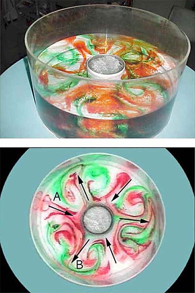
If the rotation is set at 10rpm (or indeed any rotation rate exceeding 2rpm or so), we see the development of eddies which sweep (relatively) warm fluid from the periphery to the cold can in one sector of the tank (e.g. A below) and, simultaneously, carry cold fluid from the can to the periphery at another (e.g. B below). In this way a radially-inward heat transport is achieved, offsetting the cooling at the center caused by the melting ice. These eddies are produced by the same mechanism at work in the creation of atmospheric weather systems.
The photographs below show typical flow patterns. (Top) Eddies viewed from the side with the ice can at the center. (Bottom) View from above. Eddies draw fluid from the periphery in toward the center at point A and vice-versa at point B. Here we observe three complete wavelengths around the tank. By repeating the experiment using different values of Ω, we note that the scale of the eddies decreases and the flow becomes increasingly irregular as Ω is increased. Theory tells us that the scale of the eddies depends on the rotation rate (higher rotation rate results in smaller eddies), the depth of the fluid and the stratification that is set up in the fluid.
Previously Performed Experiments
The photos below show the evolution of the flow in a fully turbulent regime when Ω=10rpm. View a movie of this experiment here.

Rossby Number on the eddy scale
Tracking of paper dots can be used to measure typical horizontal current speeds, u. It is very instructive to estimate the Rossby number, Ro = u / 2ΩL, where L is the length scale of a typical eddy – i.e. the scale of the swirls seen in the dye photographs above. Typical surface current speeds are a few mm s-1 or so, Ω is 1.0 rad s-1, and the eddy length scale is 10cm or so, yielding a Rossby number of 0.01 – thus the motion is close to geostrophic balance (except at the bottom and sides where friction becomes important).
Radial Heat Flux
The eddies transport heat radially inwards to offset cooling induced by the melting of ice. The equilibrium condition, assuming that no heat is lost to the laboratory through the upper surface or the sides (perhaps not a good assumption!), can be written thus:
where L is the latent heat of fusion for ice (333 kJ kg-1), dm is the mass of ice that melts in a time dt, ρ and cp are the density and specific heats (4.2 kJ kg-1 K-1) of water, respectively. v’T’ is the radial eddy temperature flux and the double integral is the flux integrated first vertically and then around the tank at a chosen radius.
We can estimate dm/dt by measuring the mass of ice that melts in a given time. In the experiment described here, it took 37 minutes for 1.1 kg of ice to melt in the can, implying an energy loss of 170 W. Can this be balanced by radial heat flux due to eddies in the tank, as assumed in the above equation? We can estimate the magnitude of this term by measuring typical velocity and temperature fluctuations.
The temperatures recorded over a 40 minute period by thermistors arranged in the fluid as set out below, is graphed by the colored wiggly lines in the probe temperature graph. We observe temperature fluctuations of amplitude of a degree C or so, with a period of approximately 2 minutes.

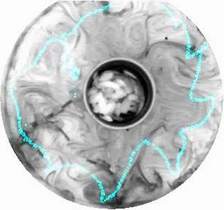
Meridional velocity perturbations were estimated by tracking a particle as it meandered around in the ice can, as shown by the blue trace in the photo below.
The v’ term was determined to be 0.6 mm s-1, at a radius of 0.20 m from the tank’s center, and taking T’ to be 0.5°C we find that the integral on the rhs of the above balance is ~ 200 W, comparable to our above estimate of the lhs of 170W. The agreement is perhaps fortuitously close but suggestive that such a balance is occurring.