Introduction | Tank – How to | Tank – Examples | Atmosphere – Examples | Theory| For Teachers | Wiki
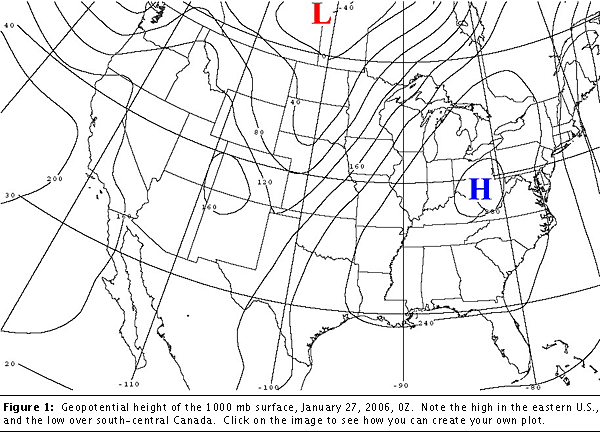
Below is a geopotential height map over the U.S. on January 27th, 2006, for the 1000 mb pressure surface. The contour interval is 40m and the labels are in meters. Maps such as these are discussed in some detail in Section 7.4 of the notes here. Note the high in the eastern U.S., and the low over south-central Canada. You can create your own plots of maps presented here simply by clicking on the image itself.
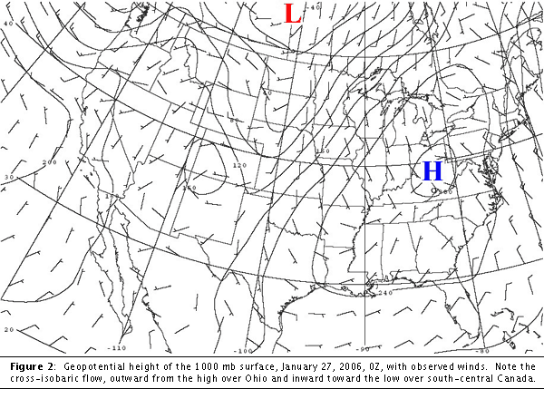
Friction in the Ekman layer causes winds to deviate toward low pressure, i.e. inward toward the low, outward from the high. The figure below shows the geopotential height of the 1000 mb surface, January 27, 2006, 0Z, with observed winds. Note the cross-isobaric flow, outward from the high over Ohio and inward toward the low over south-central Canada.
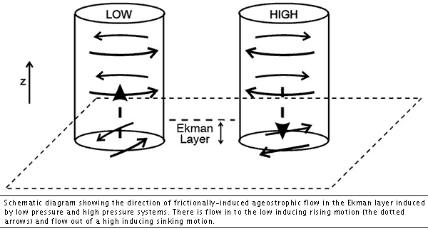
Because the horizontal flow is convergent into the low, mass continuity demands a compensating upper level outflow. This Ekman pumping near low pressure produces ascent, and this forms clouds and rain. Near a high, the divergence of the Ekman layer flow demands subsidence (Ekman suction), which is why high pressure systems tend to be characterized by clear skies. The schematic diagram that follows shows the direction of frictionally-induced ageostrophic flow in the Ekman layer induced by low pressure and high pressure systems. There is flow in to the low inducing rising motion (the dotted arrows) and flow out of a high inducing sinking motion.
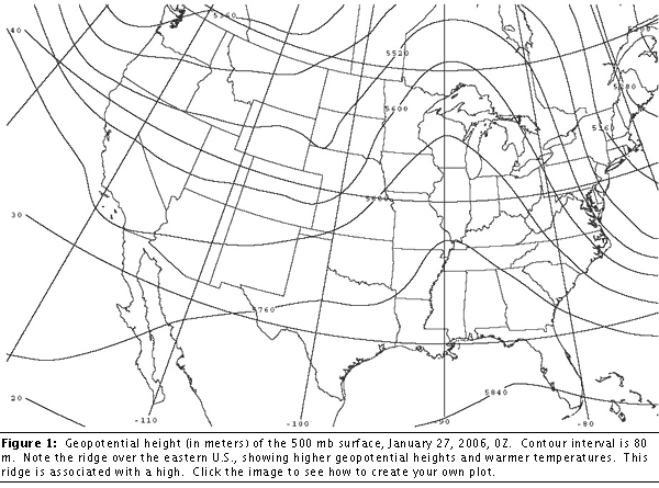
The free atmosphere exists above the Ekman layer and the effects of friction are small. Below is a map of the height of the 500 mb pressure surface over the U.S. on January 27th, 2006. It is between 5-6 km above sea level but slopes down towards the pole. Contour interval is 80 m. Note the ridge over the eastern U.S., showing higher geopotential heights and warmer temperatures. This ridge is associated with a high. Here again, simply click on an image to learn how to create your own plots
.
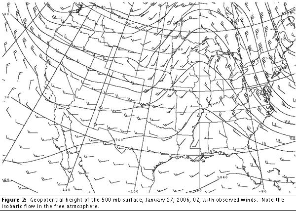
In the free atmosphere where there is little friction, winds are geostrophic, i.e. the pressure gradient and Coriolis forces balance (see Section 7.1 here for notes on geostrophic balance). Consequently, winds are aligned parallel to lines of constant pressure, clockwise around a high and counterclockwise around a low in the Northern Hemisphere. The map below shows the geopotential height of the 500 mb surface, January 27, 2006, 0Z, with observed winds. Note the isobaric flow in the free atmosphere. Maps such as these are discussed in some detail in Section 7.1 of the notes here.