Even at modest rotation rates the effect of rotation is pronounced and parcels complete many circuits before finally exiting through the drain hole. In the presence of rotation the free surface becomes markedly curved, high at the periphery and plunging downwards toward the hole in the center.
The trajectories of several particles released at different radii of the cylinder are charted in the figures below. The rotation rate was 10 rpm. Each dot marks the position of a particle every 1/10 second. The particle tracker can be used to follow individual particles or up to 10 particles simultaneously.
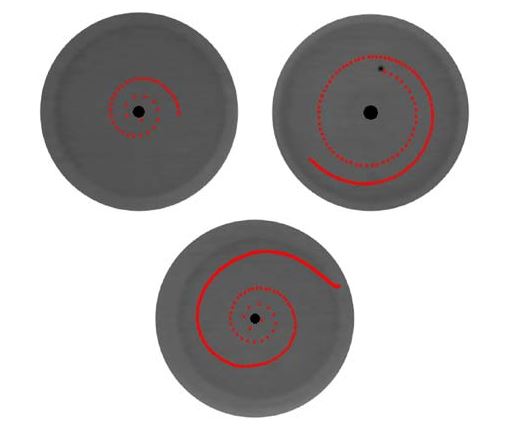
Fig.1: The trajectory of three particles released at varying distances from the drain hole. The rotation rate was 10rpm.
In Fig.2, we see the trajectory of a single particle as it moves toward the center plotted after the particle tracker data has been drawn into Excel®.
Fig. 2: Trajectory of a single particle as it circles around the drain hole at the center.
A useful way to test the data against theory is to plot the measured Rossby number defined by:
as a function of the particle’s radius. Here vθmeasured is the azimuthal speed of a particle at radius r as measured using the particle tracker. The computation of vθmeasured from the particle tracker data is discussed in detail here .
The Rossby number is a dimensionless quantity that relates the ratio of inertial forces to Coriolis forces in a rotating fluid system. At different radii from the center of the bucket, our system displays vastly different Rossby numbers. By measuring the speed of the particles as a function of radius we can experimentally determine the Rossby number.
Pictured below is a graph of experimental data obtained at a rotation rate of 20 rpm plotted against a theoretical curve that assumed angular momentum conservation, as now described.
Fig. 3: Rossby number, Ro, plotted as a function of the particle’s radius, r/r1 in the case Ω=20rpm. The continuous line is a theoretical prediction based on angular momentum conservation: the points are estimates of Ro obtained by tracking particles.
The continuous line in Fig.3 is a plot of:
and is the Ro number that would be observed if the particles conserved angular momentum – see below.
Conservation of angular momentum in radial inflow experiment
The theoretical curve in Fig.3 was deduced as follows.
Fluid setting out from the outer wall will have angular momentum because the apparatus is rotating. At r1, the radius of the bucket, fluid has velocity Ωr1 and hence angular momentum Ωr12. As parcels of fluid flow inwards they will conserve this angular momentum (provided that they are not rubbing against the bottom or the side). Thus conservation of angular momentum implies that:
where Vθ is the azimuthal velocity at radius r in the laboratory (inertial) frame given by:
where Ω is the rate of rotation of the tank in radians per second. Note that Ωr is the azimuthal speed of a particle stationary relative to the tank at radius r from the axis of rotation.
Substituting for Vθ, Eq.1 implies that
We thus see that the fluid acquires a sense of rotation which is the same as that of the rotating table but which is greatly magnified at small r. If Ω > 0 — i.e. the table rotates in an anticlockwise sense – then the fluid acquires an anticlockwise (cyclonic) swirl. If Ω < 0 the table rotates in a clockwise (anticyclonic) direction and the fluid acquires a clockwise (anticyclonic) swirl. This can be clearly seen in the trajectories shown in the examples section.
It is very instructive to test the prediction, Eq.3, by plotting up the measured Rossby number:
against the theoretical prediction
This is done in Fig.4 for various rotation rates. We see that as Ω increases the measured points and the theoretical prediction become closer to one-another, showing that the prediction (7) is increasingly good as Ω increases.
Fig.4: Measured and theoretical Rossby number plotted as a function of the particle’s radius r/r1. The continuous line is a theoretical prediction based on angular momentum conservation, Eq.(5): the points are estimates of Ro obtained by tracking particles, Eq.(4). Data is plotted from several experiments carried out at different rotation rates.
Transforming from Pixel coordinates to Cartesian and Polar coordinates
See here for more on transforming from Pixel coordinates to Cartesian and Polar coordinates.