Introduction | Tank – How to | Tank – Examples | Atmospheric- Examples | Theory | Wiki
A common example of density currents in the atmosphere is a phenomenon known as Cold Air Damming (CAD). CAD typically occurs adjacent to mountain ranges that act as barriers to air transport, as schematically shown in Fig 1.
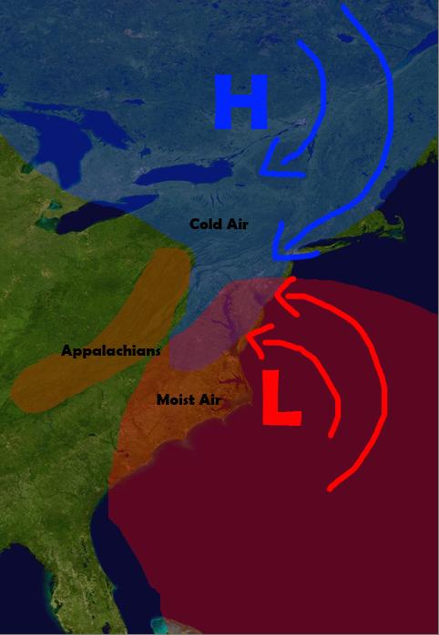
Fig. 1 Schematic diagram showing the typical surface flow associated with cold air damming. Here the Appalachians act as the dam.
(From http://en.wikipedia.org/wiki/Cold_air_damming).
Typically, a high pressure center to the north of the barrier will circulate cold, polar air southward. When the cold air reaches the mountain it is blocked and deflected along the range. Warm air within a low pressure system moving in from the south cannot replace the cold air but instead moves over it, possibly resulting in heavy precipitation.
CAD is often observed to occur during a typical Nor’easter event. Fig. 2 shows the surface conditions on February 12th, 2006 at 12GMT, when a Nor’easter is developing over Cape Hatteras. Notice that at this time, a high pressure system over Canada is advecting cold air from Quebec southward along the Eastern US coastline.
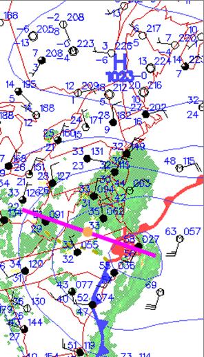
Fig. 2 Surface Conditions in the Eastern US on February 12th, 2006 at 12 GMT when a Nor’easter is developing. The purple line indicates the location of the cross-sections of potential temperature in Figs. 6 and 7. The orange dot indicates the site of the temperature profiles in Figs. 8 and 9.
Once the cold air reaches the Appalachian mountains (see Fig. 3) the mountains deflect it southward, creating a cold air wedge at low levels that sweeps parallel to the Appalachians. This in turn creates a strong inversion with cold air at the surface and warm air over it.
Fig. 3 Topography of the Eastern US. The Appalachians create a barrier for easterly flow and deflects wind southward. The red line indicates the location of the potential temperature sections of Figs 6 and 7. The blue dot shows the location of the temperature profiles of Figs 8 and 9.
The southward deflection of the cold air wedge is evident in Fig. 4., showing the observed wind at 1000 mb. Over the Atlantic Ocean, easterly winds are deflected to the south as they move inland and encounter the Appalachians shown in Figure 3.
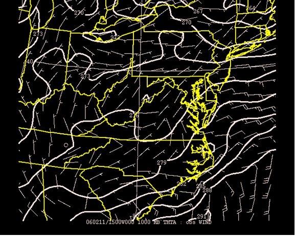
Fig. 4 Potential temperature and observed wind at 1000mb on February 11, 2006 at 3 GMT. Notice that wind is deflected southward along the Appalachians.
When looking at observed winds at the 500 mb level on February 11, 2006 at 3 GMT (Fig. 5), it is clear that CAD is a low level phenomenon. At 500 mb, there are no physical barriers and the wind has a general westerly motion with no deflection along topographical features.
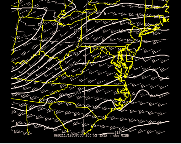
Fig. 5 Potential temperature and observed wind at 500mb on February 11, 2006 at 3 GMT.
The cold air wedge can be better illustrated using temperature sections that cut through the Appalachians. Fig. 6 shows a cross-section of potential temperature vs log pressure on February 11th, 2006 at 6 GMT, along the line marked in red Fig 2. Cold air (less than 282 K), is indicated in green. Note that at this time the warm air occupies the base of the Appalachians.
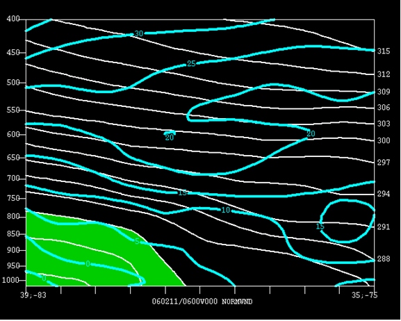
Fig. 6 Potential temperature vs. Log Pressure Along a Cross-Section from 35N, 75W to 39N, 83W on February 11, 2006 6AM UT.
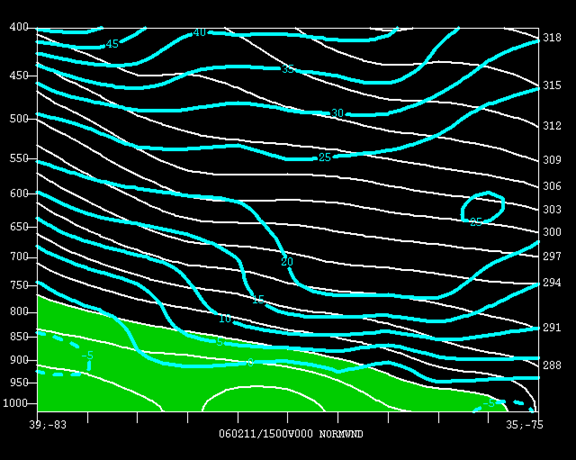
Fig. 7 Potential temperature vs. Log Pressure along a section from 35N, 75W to 39N, 83W on February 11, 2006 15 GMT.
Fig. 7 shows the same cross-section 9 hours later at 15 GMT. At this time the cold air has wedged itself below the warm air, leading to a marked wind shear up to 700 mb. The meridional wind near the surface no longer flows from the South instead it now flows from the North. This reminds us of the two opposining currents observed in the Marsigli experiment
The wedge of cold denser air under the warm air aloft can also be illustrated by looking at temperature profiles located along the base of the Appalachians. Fig. 8 shows the temperature profile at the point 37N latitude, 79W longitude (Southwestern Virginia – see blue dot in Fig. 3)
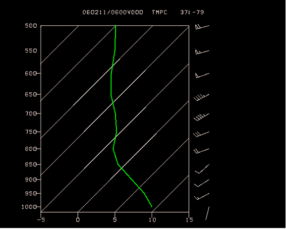
Fig. 8 On February 11, 2006 at 6 GMT. Surface is relatively warm with surface winds from the South (plotted on the right hand side).
Fig. 9 shows the temperature profile 9 hours later at 15 GMT. At this time, surface temperature decreases to 2 degrees Celsius and the layer up to 850mb is also colder. However, above 850 mb, temperatures remain nearly constant showing that a cold air is wedging itself below relatively warmer air. In addition, the surface winds had shifted in direction and now blow from the North, pushing the cold the cold air wedge southward. A very strong opposite flow is observed at 850 mb.
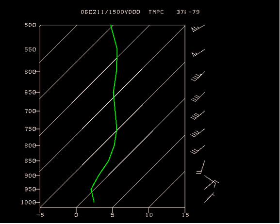
Fig. 9 Temperature vs Log Pressure Profile at 37N, 79W (Southwestern Virginia) on February 11, 2006 a 15 GMT. Surface temperatures decrease as the cold air wedge reaches the area. However, the air aloft remains relatively unchanged.