Rossby Waves – Theory

Introduction | Tank – How to  | Tank – Examples  |  Ocean – Examples  | Theory

Physical Mechanism

In the dye stirring Taylor columns experiments, it is demonstrated that a rotating fluid has a certain rigidity parallel to the axis of rotation, so that the flow is essentially two-dimensional. For slow, steady, frictionless flow (i.e. Ro << 1), taking the curl of the momentum equation gives (assuming the fluid to be barotropic, i.e. one in which ρ = ρ(p)) the Taylor-Proudman Theorem:

where u is the flow vector, Ω is the rotation vector of the motion, ρ is the density and p the pressure. Hence u does not vary in the direction parallel to Ω under the prescribed conditions.

The atmosphere and ocean are on the rapidly rotating earth, so they will be affected by the Taylor-Proudman Theorem. Consider the spherical shell of fluid sketched in Fig. 1. If the fluid were of constant density, then if Ro << 1 we know from the Taylor-Proudman theorem (see Eq.1) that rigidity will be imparted to the fluid along an axis parallel to the Earth’s rotation.

By Eq.1, the Taylor columns in the fluid cannot change their length or tip over. Thus the columns of fluid marked in Fig. 1 can readily move east-west (at least in the absence of meridional boundaries) because this doesn’t result in any change in length of the column. However, due to the sphericity of the earth, the columns cannot easily move north-south since this would imply a change in length.

Fig.1 An illustration of Taylor-Proudman on a rotating sphere. We draw a spherical shell of homogeneous fluid of constant thickness h. The length of the Taylor columns, d, aligned parallel to Ω, increase as the equator is approached.

Suppose a column from Fig.1 (or in the tank with a tilted bottom) is displaced poleward (i.e., towards the shallow end of the tank). The length of the Taylor column must be reduced, so it will be squashed, and anticyclonic vorticity induced (see Eq. 4 below). If a column is displaced equatorward, it will be stretched, inducing cyclonic vorticity (again, see Eq.4 below).

Imagine a series of Taylor columns aligned along a latitude circle (so that intially they are all of the same length). If the columns are then displaced in an undulating pattern, one poleward, the next equatorward, the next poleward, etc., then the vorticity induced by the stretching/squashing of the displaced Taylor Columns results in the phase of the undulating pattern propagating westward (see Fig. 2). This pattern is known as a Rossby wave.

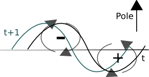
Fig.2 The sense of the relative vorticity induced by the meridional displacement of Taylor columns. The ‘+’ represents the vorticity associated with a stretched Taylor column, and the ‘-‘ represents that associated with a squashed Taylor column. The phase of the undulating vorticity pattern propagates westward.

It can be shown that, on the sphere, Rossby waves satisfy the dispersion relation

where c_p is the phase velocity, K the total wavenumber (where K² = k² + l²) and ω the frequency. Here β = df/dy [where f is the Coriolis parameter (f = 2Ωsinφ, φ the latitude) and y is a coordinate locally increasing northwards), sometimes called the planetary vorticity gradient. In the case of our laboratory experiment, β is replaced by β^* as defined in Eq.7 below.

Rossby waves in the ‘ice cube’ experiments

Fig.3 Schematic of the motion of an ice cube in the rotating frame of reference of the tank for the sloped plane experiment. The path represents the flow near the ice cube as the ice moves to the left (“west”). Note x points east, and y points poleward. The trajectory has been exaggerated. Click here to see actual trajectories.

The cone and plane ‘ice cube’ experiments simulate the change in length of the Taylor columns by varying the depth of the rotating tank – the shallow area of the tank represents the (north) pole, and the deeper area represents the equator. Cold water from the ice cube sinks, causing water to be drawn towards the cube. Conservation of angular momentum means that the ice cube begins to rotate relative to the tank in the direction of the tank’s rotation, hence generating a cyclonic circulation. This pushes fluid close to the ice cube up or down the slope depending on whether the fluid is to the “West” or the “East” of the ice cube. Hence the Taylor columns are compressed or stretched, leading to the generation of vorticity, and a Rossby wave.

Fig.4 Schematic of the motion of an ice cube in the rotating frame of reference of the tank in the cone experiment. The path represents the flow near the ice cube as the ice moves to the “west”. The trajectory has been exaggerated. Click here to see actual trajectories.

‘Ice cube’ experiment theory

We focus on the sloped plane experiment in the investigation of the theory. We can derive a relation analagous to the dispersion relation in Eqn. 2 for our rotating tank. From Ertel’s theorem applied to shallow water, we have that potential vorticity is conserved:

where u is the flow vector, Ω the rotation vector, and H the local depth of the fluid. Hence, for small Rossby number flow (i.e., ∇ x u << Ω)

Note that if DH/Dt < 0, we have in the vertical direction that D(∇ x u)/Dt|_k < 0, so anticyclonic vorticity is induced. Similarly, if DH/Dt > 0 (fluid column stretched), D(∇ x u)/Dt|_k > 0, and cyclonic vorticity is induced, confirming our physical argument.

Now, taking y to be the coordinate in the direction of decreasing depth (in a “northwards” direction as in the northern hemisphere), we can write

Putting this back into equation 3, linearising D/Dt(∇ x u) and looking at the vertical components, we have:

Here β^* = (gradient of tank depth) x 2Ω / H where Ω is the magnitude of the rotation vector, and H the local depth of the tank. It is the analogue of β = df/dy on the sphere.

Introducing a streamfunction for the flow, ψ, Eq.6 can be written as the Rossby Wave Equation:

where x points eastwards along constant depth contours.
(Here ∇² = ∂²/∂x² + ∂²/∂y²)
Seeking solutions of the form ψ = ψ̃ e^{i(kx + ly – ωt)}, we arrive at the dispersion relation Eq.2 with β^*= β

Setting k = l, λ = 2π/k, we derive an expression for the phase speed which can be applied for our tank experiment:

If we investigate the dispersion relation for the ice cube rotation (eqn. 2), substituting in Ω ≈ π / 2 s^-1, H ≈ 0.05m and a slope ≈ 0.5 gives:

So for the generated Rossby waves (of wavelength around 0.05m), c_p is of the order of 0.001ms^-1, i.e., 1mm / s – roughly as seen in our experiment.

Following similar steps to these for the ‘ice cube on a cone’ experiment (using polar coordinates), the expression for the phase speed of the waves in the cone experiment is precisely Eq.9. Hence c_p is again of the order of 0.001ms^-1.