Introduction | Tank – How to | Tank – Examples | Atmosphere – Examples | Ocean – Examples | Theory | For Teachers | Wiki
Here we present some atmospheric phenomena that have contact points to the dye stirring experiment. In each example it is instructive to estimate the Rossby number and so determine to what extent the earth’s rotation plays a role – see theory section for definition and discussion of the Rossby number.
Chernobyl
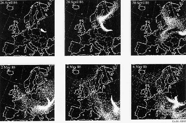
On April 26, 1986, at 1:23A.M., the world’s worst nuclear power accident occurred at Chernobyl in the former USSR (now Ukraine). A chain reaction in one of the four reactors span out of control, blowing off the reactor’s lid and killing dozens of people instantly. Many others had to be evacuated from the surrounding area. A plume of radioactive particles was ejected into the atmosphere.
Two maps are shown above charting the evolution of the plume over Europe. Note how regions many hundreds of kilometers to the northwest, during the first two days after the disaster, received more radiation than areas only slightly to the east. If the two snapshots shown above were taken exactly 48 hours apart, estimate the Rossby number of the large-scale flow advecting the plume. Is it small or large, and what does this tell us?
The image below shows the evolution of the plume over a 10-day period.
California Wildfires
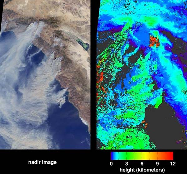
Santa Ana winds are fast moving, warm air currents that blow out of the deserts of California toward the coast. They are formed from high pressure forcing air down-slope, with warming due to adiabatic descent (compression due to increase in pressure doing work on the air parcels, so warming them up). Such winds can have a drying effect on vegetation, increasing the chance of wildfire. The above images show smoke from a series of wildfires near the Californian coast showing smoke being blown by Santa Ana winds. Much like the Chernobyl plume maps, the smoke from the wildfires is carried along by the prevailing winds. Estimate the Rossby number, assuming a typical wind speed of 10 m s-1. How does it compare to the Chernobyl example?
Water Vapor in the Atmosphere
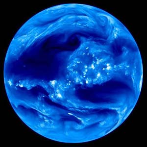
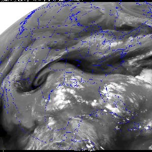
Images of the water vapor distribution in the atmosphere are a vivid illustration of how large-scale flow in the atmosphere stirs tracers around the globe. Note the sharp gradients of water vapor concentration in the atmosphere revealed by the boundaries between darker (dry) and brighter (moist) areas. A movie showing the movement of water vapor over Antartica is available here. For the N Hemisphere see here.
Estimate the Rossby number, assuming a typical wind speed of 10 m s-1. How does it compare to the above examples?
Jupiter
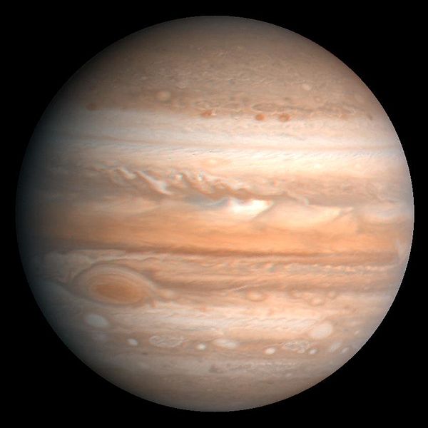
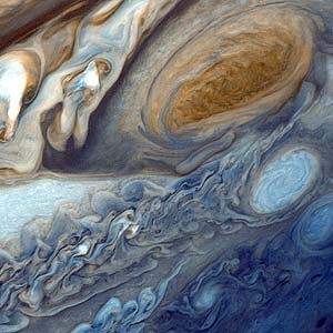
Jupiter images from Voyager 1. On the right, a false-colour image of the Great Red Spot of Jupiter. NASA image.
Jupiter, like Earth, is a rapidly-rotating planet, making a complete rotation in only 9.8 Earth hours. Yet is has a radius that is more than 11 times that of the earth! Because of this rapid rotation, Jupiter’s atmosphere is under strong rotational control. Note the qualitative similarities between the tracer patterns in our dye-stirring experiment and the patterns evident in Jupiter’s atmosphere, such as the Giant Red Spot (right).
Estimate Jupiter’s planetary Rossby number (at 45ÜN), assuming a typical wind speed of 150 m s-1. How does it compare to Earth’s atmosphere and the Rossby number estimated in our dye stirring experiment on the rotating table?